DensityPlot#

class pycafee.normalitycheck.densityplot.DensityPlot(language=None, **kwargs)[source]#

Methods

`draw`(x_exp[, ax, bw_method, which, x_label, ...])	This function draws the non-parametric density plot with the option to add the central tendency measurements
`get_language`()	Returns the current language
`set_language`(language)	Changes the current language

draw(x_exp, ax=None, bw_method=None, which=None, x_label=None, y_label=None, width='default', height='default', export=None, file_name=None, extension=None, dpi=None, tight=None, transparent=None, plot_design='gray', legend=None, decimal_separator=None)[source]#

This function draws the non-parametric density plot with the option to add the central tendency measurements

Parameters

x_exp1D numpy array

The data to be fitted

axNone or matplotlib.axes.SubplotBase

If ax is None, a figure is created with a preset design. The other parameters can be used to edit and export the graph.
If ax is a matplotlib.axes.SubplotBase, the function returns a matplotlib.axes.SubplotBase with the DensityPlot axis. In this case, only the which and bw_method parameters affect the plot.

bw_methodstr, optional

The method used to calculate the estimator bandwidth. This can be "scott" or "silverman". If None (default), the "scott" method is used. This is the bw_method parameter from scipy.stats.gaussian_kde(), but limited to "scott" or "silverman" options. For other options, use the original method [1].

whichstr, optional

The parameter which controls which measures of central tendency should be added to the graph. The options are:

None (default): no measures of central tendency are included;
"mean": adds the mean;
"median": adds the median;
"mode": adds the mode(s) (only if the data has a mode);
"all": adds the mean, median and the mode(s) (if the data das a mode);

To add two measures of central tendency, combine their names separated by a comma (","). For example, to add the mean and the median, use which = "mean,median".

legendbool, optional

Whether the legend should be added into the chart (True) or not (False). The default value is None, which implies True.

x_labelstr, optional

The label to be displayed on x label. Default is None, which results in "data".

y_labelstr, optional

The label to be displayed on y label. Default is None, which results in "Non-parametric density".

width"default", int or float (positive), optional

The width of the figure. If it is "default", it uses a pre-defined value. If it is a number, it defines the width of the chart (in inches).

height"default", int or float (positive), optional

The height of the figure. If it is "default", it uses a pre-defined value. If it is a number, it defines the height of the chart (in inches).

exportbool, optional

Whether the graph should be exported (True) or not (False). The default value is None, which implies False.

file_namestr, optional

The file name. Default is None which results in a file named "kernal_density".

extensionstr, optional

The file extension without a dot. Default is None which results in a ".png" file.

dpiint or float (positive), optional

The figure pixel density. The default is None, which results in a 100 dpis picture. This parameter must be a number higher than zero.

tightbool, optional

Whether the graph should be tight (True) or not (False). The default value is None, which implies True.

transparentbool, optional

Whether the background of the graph should be transparent (True) or not (False). The default value is None, which implies False (white).

plot_designstr or dict, optional

The plot desing. If "gray", uses a gray-scale desing (default). If "colored", uses a colored desing. If dict, it must have five keys ("kde", "Mean", "Median", "Mode", "Area"), where each one defines the design of each element added to the chart.

decimal_separatorstr, optional

The decimal separator symbol used in the chart. It can be the dot (None or ".") or the comma (",").

Returns

kde_xnumpy array: The x values used to plot the graph
kde_ynumpy array: The y values used to plot the graph
central_tendencydict: A dictionary with the measures of central tendency of the data with respective value estimated by the kde function.
axesmatplotlib.axes._subplots.AxesSubplot: The axis of the graph.

See also

pycafee.normalitycheck.dotplot.DotPlot.draw

Notes

The plot_design paramter must be a dict where the values for all keys must be a list. The lists of the keys "kde", "Mean", "Median", and "Mode" must have:

the first element must be a str with the color name;

the second element must be a str with line style;

the third element must be a number (int or float, positive) with the line thickness.

The Area list must have a single element, which is a str with the name of the color that fills the area between the fit and the line y = 0. For example:

plot_design = {
    "kde": ['k', '-', 1.5],
    "Mean": ['dimgray', '--', 1.5],
    "Median": ['darkgray', '--', 1.5],
    "Mode": ['lightgray', '--', 1.5],
    "Area": ['white'],
}

☕

To obtain which extensions the figure can be exported, use the following script:

>>> from matplotlib import pyplot as plt
>>> suported_types = plt.gcf().canvas.get_supported_filetypes()
>>> for key, value in suported_types.items():
        print(key, ":", value)
>>> plt.close()

The mode is calculated using the multimode function.

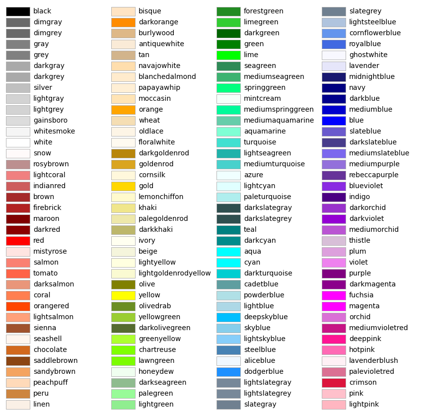
A list of color names can be found at matplotlib’s documentation.

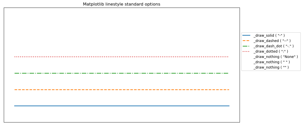
A list of linestyles can be found here.

References

1: SCIPY. scipy.stats.gaussian_kde. Available at: www.scipy.org. Access on: 10 May. 2022.

Examples

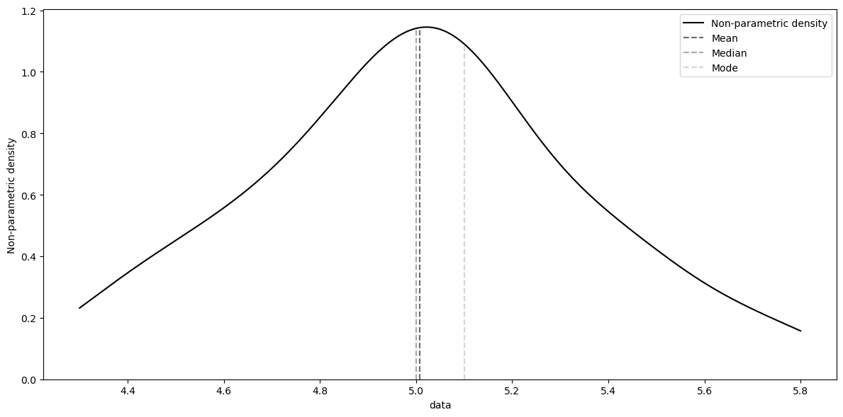
Nonparametric density plot with default parameters plus the measures of central tendency.

>>> from pycafee.normalitycheck.densityplot import DensityPlot
>>> import numpy as np
>>> x_exp = np.array([
            5.1, 4.9, 4.7, 4.6, 5.0, 5.4, 4.6, 5.0, 4.4, 4.9, 5.4, 4.8, 4.8, 4.3, 5.8, 5.7, 5.4, 5.1, 5.7,
            5.1, 5.4, 5.1,4.6, 5.1, 4.8, 5.0, 5.0, 5.1, 5.2, 5.2, 4.7, 4.8, 5.4, 5.2, 5.5, 4.9, 5.0, 5.5, 4.9, 4.4,
            5.1, 5.0, 4.5, 4.4, 5.0, 5.1,4.8, 5.1, 4.6, 5.3, 5.0
            ])
>>> densityplot = DensityPlot()
>>> densityplot.draw(x_exp, which="all", export=True)
    The 'kernal_density.png' file was exported!

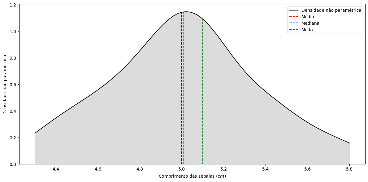
Nonparametric density with some editing

>>> from pycafee.normalitycheck.densityplot import DensityPlot
>>> import numpy as np
>>> x_exp = np.array([
            5.1, 4.9, 4.7, 4.6, 5.0, 5.4, 4.6, 5.0, 4.4, 4.9, 5.4, 4.8, 4.8, 4.3, 5.8, 5.7, 5.4, 5.1, 5.7,
            5.1, 5.4, 5.1,4.6, 5.1, 4.8, 5.0, 5.0, 5.1, 5.2, 5.2, 4.7, 4.8, 5.4, 5.2, 5.5, 4.9, 5.0, 5.5, 4.9, 4.4,
            5.1, 5.0, 4.5, 4.4, 5.0, 5.1,4.8, 5.1, 4.6, 5.3, 5.0
            ])
>>> densityplot = DensityPlot(language="pt-br")
>>> densityplot.draw(x_exp, which="all", export=True, file_name="my_data", plot_design="colored", x_label="Comprimento das sépalas ($cm$)")
    O arquivo 'my_data.png' foi exportado!

get_language()#: Returns the current language

set_language(language)#

Changes the current language

Parameters

languagestr: The language code

Notes

The language must be a str with no more then 5 elements.

DotPlot

Sample